Note
This tutorial was generated from a Jupyter notebook that can be downloaded here.
Using gwent to Calculate Signal-to-Noise Ratios
Here we present a tutorial on how to use gwent to calculate SNRs for
the instrument models currently implemented (LISA, PTAs, aLIGO, and
Einstein Telescope) with the signal being an array of coalescing Binary
Black Holes.
First, we import important modules.
import numpy as np
import matplotlib.pyplot as plt
import matplotlib as mpl
from scipy.constants import golden_ratio

import astropy.constants as const
import time
import astropy.units as u

import gwent
import gwent.binary as binary
import gwent.detector as detector
import gwent.snr as snr
from gwent.snrplot import Plot_SNR

#Turn off warnings for tutorial
import warnings
warnings.filterwarnings('ignore')
Setting matplotlib preferences and adding a pretty plot function for fig sizes
def get_fig_size(width=7,scale=2.0):
    #width = 3.36 # 242 pt
    base_size = np.array([1, 1/scale/golden_ratio])
    fig_size = width * base_size
    return(fig_size)
mpl.rcParams['figure.dpi'] = 300
#mpl.rcParams['figure.figsize'] = get_fig_size()
mpl.rcParams['text.usetex'] = True
mpl.rc('font',**{'family':'serif','serif':['Times New Roman']})
mpl.rcParams['lines.linewidth'] = 1.3
mpl.rcParams['axes.labelsize'] = 12
mpl.rcParams['xtick.labelsize'] = 10
mpl.rcParams['ytick.labelsize'] = 10
mpl.rcParams['legend.fontsize'] = 8
We need to get the file directories to load in the instrument files.
load_directory = gwent.__path__[0] + '/LoadFiles/InstrumentFiles/'
Fiducial Source Creation
To run snr.Get_SNR_Matrix, you need to instantiate a source. Since
we need to reinitialize a few times, we just put it here as a function.
This is an example for reasonable mass ranges for the particular detector mass regime and the variable ranges limited by the waveform calibration region.
The source parameters must be set (ie. M,q,z,chi1,chi2), but one also
needs to set the minima and maxima of the selected SNR axes variables.
This takes the form of
source_param = [fiducial_value,minimum,maximum]
def Initialize_Source(instrument,approximant='pyPhenomD',lalsuite_kwargs={}):
    """Initializes a source binary based on the instrument type and returns the source

    Parameters
    ----------
    instrument : object
        Instance of a gravitational wave detector class
    approximant : str, optional
        the approximant used to calculate the frequency domain waveform of the source.
        Can either be the python implementation of IMRPhenomD ('pyPhenomD', the default) given below,
        or a waveform modelled in LIGO's lalsuite's lalsimulation package.
    lalsuite_kwargs: dict, optional
        More specific user-defined kwargs for the different lalsuite waveforms
    """

    #q = m2/m1 reduced mass
    q = 1.0
    q_min = 1.0
    q_max = 18.0
    q_list = [q,q_min,q_max]

    #Chi = S_i*L/m_i**2, spins of each mass i
    chi1 = 0.0 #spin of m1
    chi2 = 0.0 #spin of m2
    chi_min = -0.85 #Limits of PhenomD for unaligned spins
    chi_max = 0.85
    chi1_list = [chi1,chi_min,chi_max]
    chi2_list = [chi2,chi_min,chi_max]

    #Redshift
    z_min = 1e-2
    z_max = 1e3

    if isinstance(instrument,detector.GroundBased):
        #Total source mass
        M_ground_source = [10.,1.,1e4]
        #Redshift
        z_ground_source = [0.1,z_min,z_max]

        source = binary.BBHFrequencyDomain(M_ground_source,
                                           q_list,
                                           z_ground_source,
                                           chi1_list,
                                           chi2_list,
                                           approximant=approximant,
                                           lalsuite_kwargs=lalsuite_kwargs)
    elif isinstance(instrument,detector.SpaceBased):
        M_space_source = [1e6,1.,1e10]
        z_space_source = [1.0,z_min,z_max]
        source = binary.BBHFrequencyDomain(M_space_source,
                                           q_list,
                                           z_space_source,
                                           chi1_list,
                                           chi2_list,
                                           approximant=approximant,
                                           lalsuite_kwargs=lalsuite_kwargs)
    elif isinstance(instrument,detector.PTA):
        M_pta_source = [1e9,1e8,1e11]
        z_pta_source = [0.1,z_min,z_max]
        source = binary.BBHFrequencyDomain(M_pta_source,
                                           q_list,
                                           z_pta_source,
                                           chi1_list,
                                           chi2_list,
                                           approximant=approximant,
                                           lalsuite_kwargs=lalsuite_kwargs)
    return source
Create SNR Matrices and Samples for a Few Examples
The variables for either axis in the SNR calculation can be:
- GLOBAL:
T_obs- Detector Observation Time
- SOURCE:
M- Mass (Solar Units)q- Mass Ratiochi1- Dimensionless Spin of Black Hole 1chi2- Dimensionless Spin of Black Hole 2z- Redshift
- GroundBased ONLY:
- Any single valued variable in list of params given by:
instrument_GroundBased.Get_Noise_Dict() - To make variable in SNR, declare the main variable, then the
subparameter variable as a string e.g.
var_x = Infrastructure Length, the case matters.
- Any single valued variable in list of params given by:
- SpaceBased ONLY:
L- Detector ArmlengthA_acc- Detector Acceleration NoiseA_IFO- Detector Optical Metrology Noisef_acc_break_low- The Low Acceleration Noise Break Frequencyf_acc_break_high- The High Acceleration Noise Break Frequencyf_IFO_break- The Optical Metrology Noise Break Frequency
- PTA ONLY:
n_p- Number of Pulsarssigma- Root-Mean-Squared Timing Errorcadence- Observation Cadence
Instrument Creation Examples
For each instrument one wants to investigate, you have to assign the fiducial noise and detector values. We do the same reinitialization game here as the source, so each of these are functions.
These examples only assign ranges of calculation for quick variable calculations, but one only needs to set the minima and maxima if they wish to use other selected SNR axes variables.
If loading a detector, the file should be frequency in the first column and either strain, effective strain noise spectral density, or amplitude spectral density in the second column.
The strain tutorial goes into more detail on initializing detectors, so if you get lost, look there!
Ground Based Detectors
def Initialize_aLIGO():
    #Observing time in years
    T_obs_ground_list = [4*u.yr,1*u.yr,10*u.yr]
    #aLIGO
    noise_dict_aLIGO = {'Infrastructure':
                  {'Length':[3995,2250,4160]},
                  'Laser':
                  {'Power':[125,10,1e3]},
                  'Seismic':
                  {'Gamma':[0.8,0.1,1.0]}}
    aLIGO = detector.GroundBased('aLIGO',T_obs_ground_list,noise_dict=noise_dict_aLIGO)

    return aLIGO
Space Based Detectors
def Initialize_LISA():
    #Values taken from the ESA L3 proposal, Amaro-Seaone, et al., 2017 (https://arxiv.org/abs/1702.00786)
    T_obs_space_list = [4*u.yr,1*u.yr,10*u.yr]

    #armlength in meters
    L = 2.5e9*u.m
    L_min = 1.0e7*u.m
    L_max = 1.0e11*u.m
    L_list = [L,L_min,L_max]

    #Acceleration Noise Amplitude
    A_acc = 3e-15*u.m/u.s/u.s
    A_acc_min = 1e-16*u.m/u.s/u.s
    A_acc_max = 1e-14*u.m/u.s/u.s
    A_acc_list = [A_acc,A_acc_min,A_acc_max]

    #The Low Acceleration Noise Break Frequency
    f_acc_break_low = .4*u.mHz.to('Hz')*u.Hz
    f_acc_break_low_min = .1*u.mHz.to('Hz')*u.Hz
    f_acc_break_low_max = 1.0*u.mHz.to('Hz')*u.Hz
    f_acc_break_low_list = [f_acc_break_low,f_acc_break_low_min,f_acc_break_low_max]

    #The High Acceleration Noise Break Frequency
    f_acc_break_high = 8.*u.mHz.to('Hz')*u.Hz
    f_acc_break_high_min = 1.*u.mHz.to('Hz')*u.Hz
    f_acc_break_high_max = 10.*u.mHz.to('Hz')*u.Hz
    f_acc_break_high_list = [f_acc_break_high,f_acc_break_high_min,f_acc_break_high_max]

    #The Optical Metrology Noise Break Frequency
    f_IFO_break = 2.*u.mHz.to('Hz')*u.Hz
    f_IFO_break_min = 1.*u.mHz.to('Hz')*u.Hz
    f_IFO_break_max = 10.*u.mHz.to('Hz')*u.Hz
    f_IFO_break_list = [f_IFO_break,f_IFO_break_min,f_IFO_break_max]

    #Detector Optical Metrology Noise
    A_IFO = 10e-12*u.m
    A_IFO_min = 1.0e-13*u.m
    A_IFO_max = 1.0e-10*u.m
    A_IFO_list = [A_IFO,A_IFO_min,A_IFO_max]

    #Unresolved Galactic WD Background
    Background = False

    #Numerical Transfer Function
    T_type = 'N'

    LISA_prop1 = detector.SpaceBased('LISA_prop1',
                                     T_obs_space_list,L_list,A_acc_list,
                                     f_acc_break_low_list,f_acc_break_high_list,
                                     A_IFO_list,f_IFO_break_list,
                                     Background=Background,T_type=T_type)
    return LISA_prop1
PTA Detectors
def Initialize_NANOGrav():
    #NANOGrav calculation using 11.5yr parameters https://arxiv.org/abs/1801.01837
    #Observing time in years
    T_obs_ptas_list = [11.42*u.yr,5*u.yr,30*u.yr]
    #rms timing residuals in seconds
    sigma = 100*u.ns.to('s')*u.s
    sigma_min = 100*u.ns.to('s')*u.s
    sigma_max = 500*u.ns.to('s')*u.s
    sigma_list = [sigma,sigma_min,sigma_max]
    #Number of pulsars
    n_p = 34
    n_p_min = 18
    n_p_max = 200
    n_p_list = [n_p,n_p_min,n_p_max]
    #Avg observation cadence of 1 every 2 weeks in num/year
    cadence = 1/(2*u.wk.to('yr')*u.yr)
    cadence_min = 2/u.yr
    cadence_max = 1/(u.wk.to('yr')*u.yr)
    cadence_list = [cadence,cadence_min,cadence_max]

    #NANOGrav 11.4 yr WN only
    NANOGrav_WN = detector.PTA('NANOGrav_WN',n_p_list,T_obs=T_obs_ptas_list,sigma=sigma_list,cadence=cadence_list)
    return NANOGrav_WN
SNR Calculations
To actually sample the parameter space, one needs to declare x and y variables that correspond to the variables inside the relavant instrument and/or model for the SNR Calculation.
You will also need to assign Sample Rates for each, this will directly determine how long a calculation will take. I have kept all curves under 100 for paper figures, so I would recommend nothing over that, but I won’t tell you what to do!
#Number of SNRMatrix rows
sampleRate_y = 100
#Number of SNRMatrix columns
sampleRate_x = 100
We now use Get_SNR_Matrix with the variables given and the data
range to sample the space either logrithmically or linearly based on the
selection of variables. It computes the SNR for each value, then returns
the variable ranges used to calculate the SNR for each matrix, then
returns the SNRs with size of the sampleRate_xXsampleRate_y
aLIGO
Varying Source Parameters
Here we calculate the SNR for three source parameters chi1,q,
and z using Get_SNR_Matrix. For ease of the example, we just do
them all at once.
#Variable on y-axis
var_ys = ['chi1','q','z']
#Variable on x-axis
var_x = 'M'
instrument = Initialize_aLIGO()
sample_x_array = []
sample_y_array = []
SNR_array = []
for var_y in var_ys:
    source = Initialize_Source(instrument)
    start = time.time()
    [sample_x,sample_y,SNRMatrix] = snr.Get_SNR_Matrix(source,instrument,
                                                       var_x,sampleRate_x,
                                                       var_y,sampleRate_y)
    end = time.time()
    sample_x_array.append(sample_x)
    sample_y_array.append(sample_y)
    SNR_array.append(SNRMatrix)

    print('Model: ',instrument.name + '_' + var_x + '_vs_' + var_y,',',' done. t = : ',end-start)
Model:  aLIGO_M_vs_chi1 ,  done. t = :  31.16754937171936
Model:  aLIGO_M_vs_q ,  done. t = :  31.795299530029297
Model:  aLIGO_M_vs_z ,  done. t = :  23.489653825759888
Plotting SNRs
This is just an example of plotting the above SNRs using the
Plot_SNR function. The function can take a ton of parameters, but
for simple plots most of them are unneccessary.
fig, axes = plt.subplots(1,3,figsize=get_fig_size())
loglevelMax=4.0
hspace = .1
wspace = .45
for i,ax in enumerate(axes):
    if i == (len(axes)-1):
        Plot_SNR('M',sample_x_array[i],var_ys[i],
                 sample_y_array[i],SNR_array[i],
                 fig=fig,ax=ax,display=True,display_cbar=True,
                 logLevels_max=loglevelMax,
                 hspace=hspace,wspace=wspace,
                 xticklabels_kwargs={'rotation':70,'y':0.02},
                 ylabels_kwargs={'labelpad':-5})
    else:
        Plot_SNR('M',sample_x_array[i],var_ys[i],
                 sample_y_array[i],SNR_array[i],
                 fig=fig,ax=ax,display=False,display_cbar=False,
                 logLevels_max=loglevelMax,
                 hspace=hspace,wspace=wspace,xticklabels_kwargs={'rotation':70,'y':0.02})
    i += 1
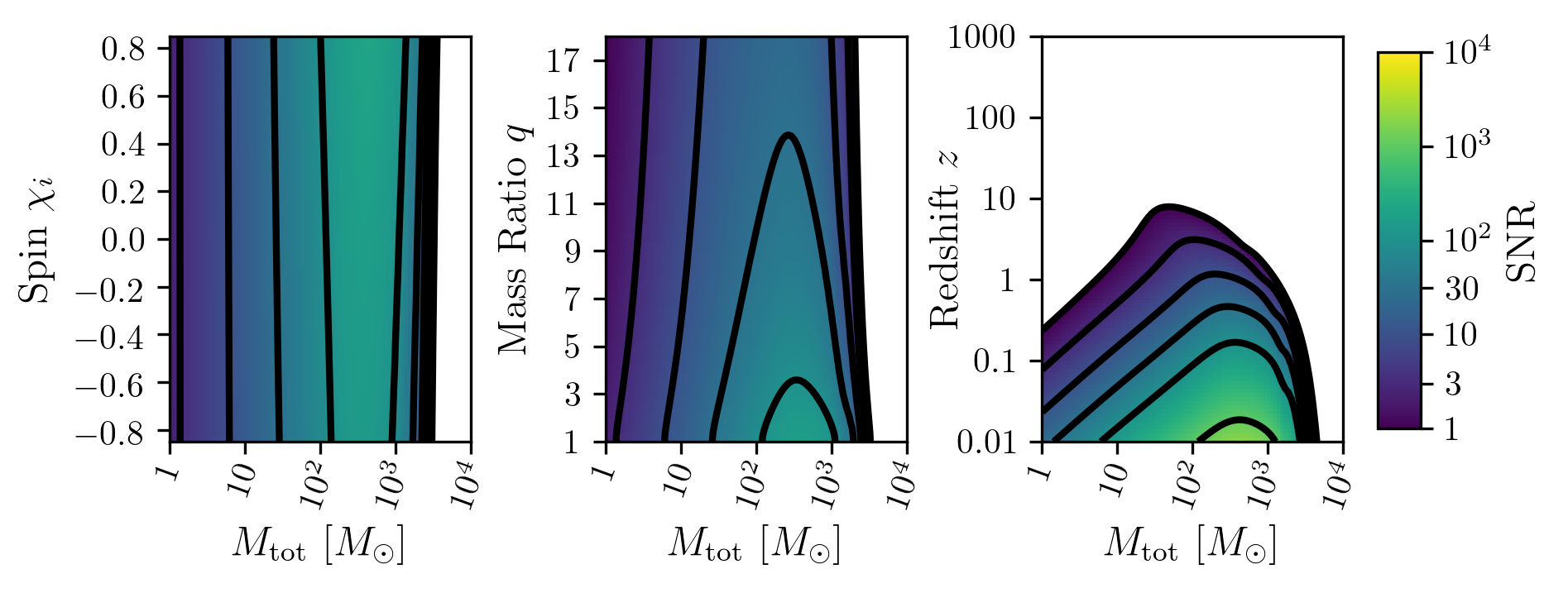
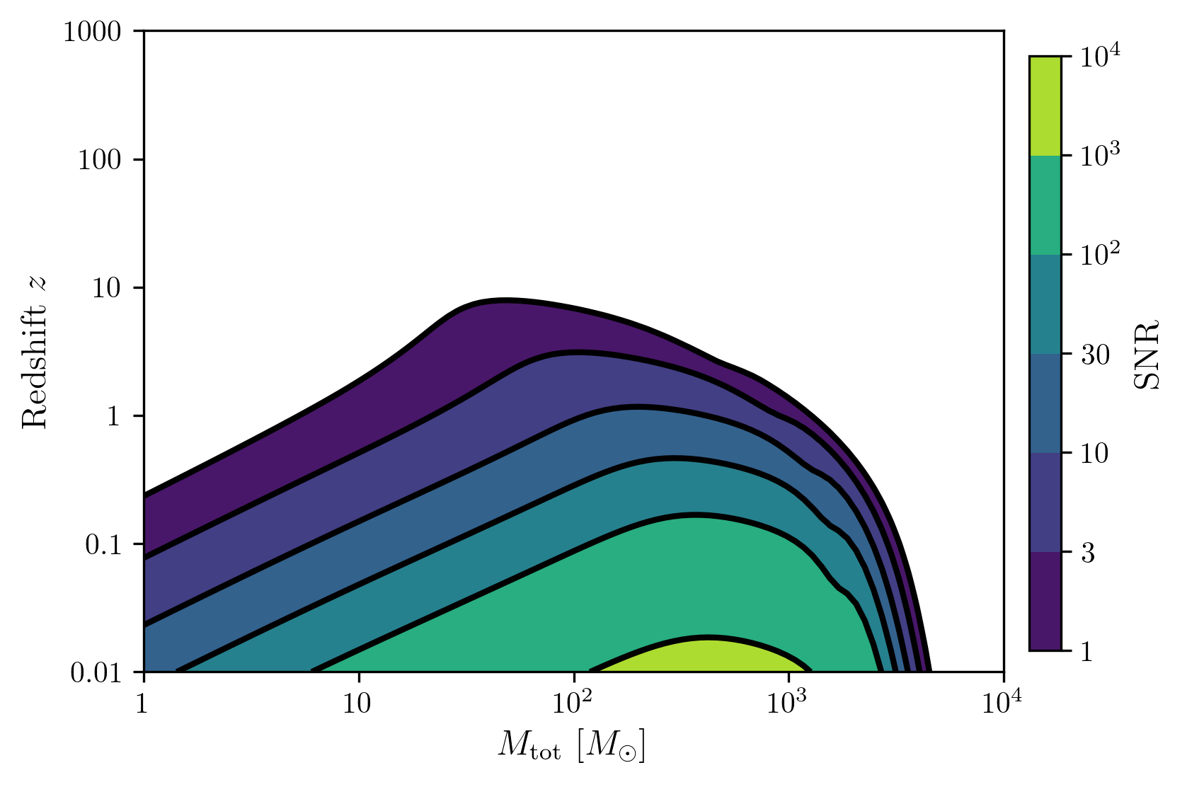
A simple example for just one figure.
Plot_SNR('M',sample_x_array[-1],'z',sample_y_array[-1],SNR_array[-1],smooth_contours=False)
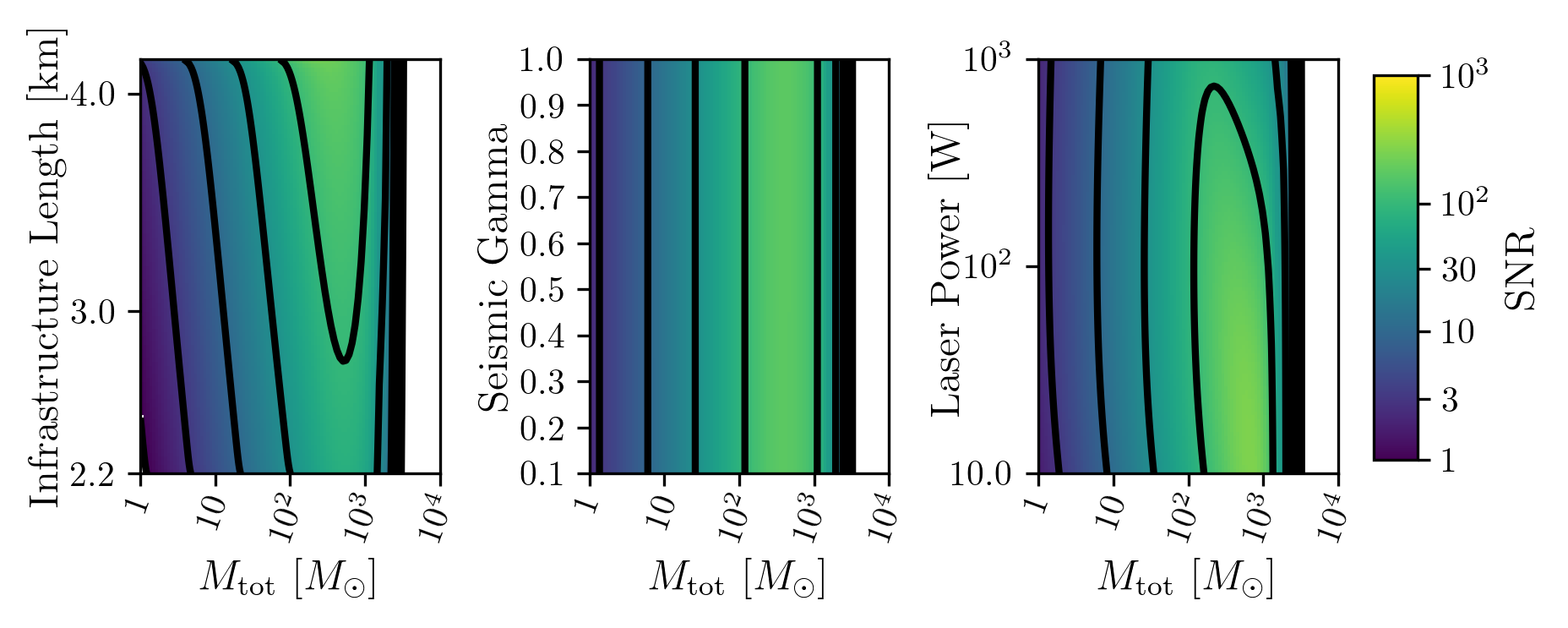
Varying Instrument Parameters
This is very similar to the previous example, but with varying the
instrument parameters Infrastructure Length, Seismic Gamma, and
Laser Powervs. M.
One thing to note is that we moved the instrument initialization inside the for loop this time since we don’t want the parameters to stay at the max value from the previous run.
#Variable on y-axis
var_ys = ['Infrastructure Length','Seismic Gamma','Laser Power']
#Variable on x-axis
var_x = 'M'
sample_x_array = []
sample_y_array = []
SNR_array = []
for var_y in var_ys:
    instrument = Initialize_aLIGO()
    source = Initialize_Source(instrument)
    start = time.time()
    [sample_x,sample_y,SNRMatrix] = snr.Get_SNR_Matrix(source,instrument,
                                                       var_x,sampleRate_x,
                                                       var_y,sampleRate_y)
    end = time.time()
    sample_x_array.append(sample_x)
    sample_y_array.append(sample_y)
    SNR_array.append(SNRMatrix)

    print('Model: ',instrument.name + '_' + var_x + '_vs_' + var_y,',',' done. t = : ',end-start)
Model:  aLIGO_M_vs_Infrastructure Length ,  done. t = :  24.8679461479187
Model:  aLIGO_M_vs_Seismic Gamma ,  done. t = :  23.985658407211304
Model:  aLIGO_M_vs_Laser Power ,  done. t = :  24.44096326828003
figsize = get_fig_size()
fig, axes = plt.subplots(1,3,figsize=figsize)
loglevelMax=3.0

wspace = .5

for i,ax in enumerate(axes):
    if i == (len(axes))-1:
        Plot_SNR('M',sample_x_array[i],var_ys[i],
                 sample_y_array[i],SNR_array[i],
                 fig=fig,ax=ax,display=True,display_cbar=True,
                 logLevels_max=loglevelMax,
                 hspace=hspace,wspace=wspace,
                 xticklabels_kwargs={'rotation':70,'y':0.02},ylabels_kwargs={'labelpad':-5})
    else:
        Plot_SNR('M',sample_x_array[i],var_ys[i],
                 sample_y_array[i],SNR_array[i],
                 fig=fig,ax=ax,display=False,display_cbar=False,
                 logLevels_max=loglevelMax,
                 xticklabels_kwargs={'rotation':70,'y':0.02},
                 ylabels_kwargs={'labelpad':1})
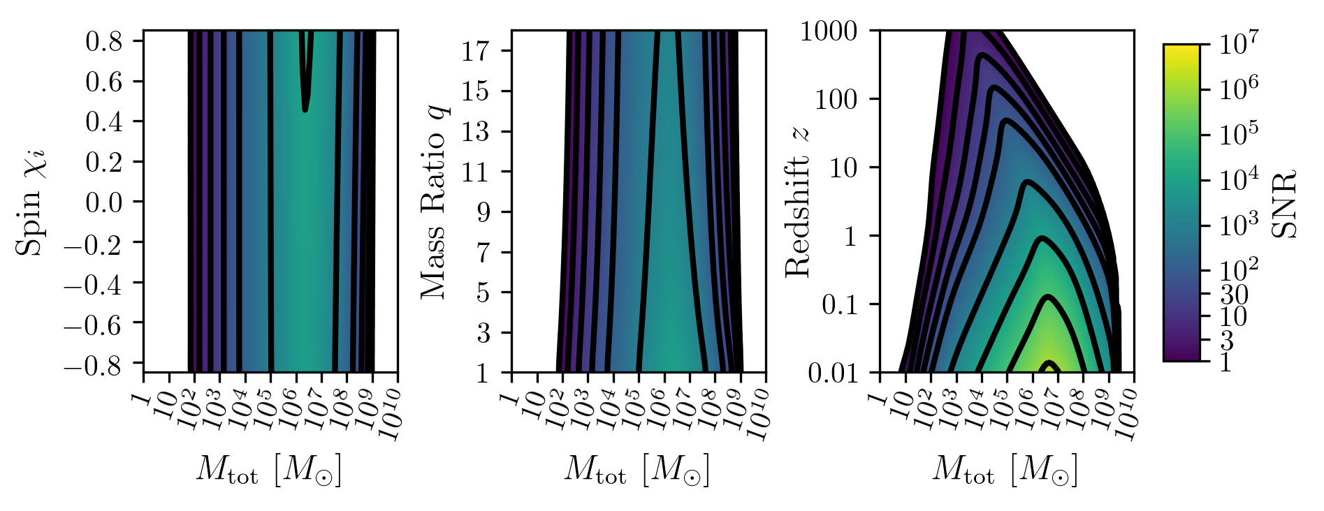
LISA SNR
We now just for examples repeat the above few SNR calculations for LISA parameters.
#Variable on y-axis
var_ys = ['chi1','q','z']
#Variable on x-axis
var_x = 'M'
instrument = Initialize_LISA()
sample_x_array = []
sample_y_array = []
SNR_array = []
for var_y in var_ys:
    source = Initialize_Source(instrument)
    start = time.time()
    [sample_x,sample_y,SNRMatrix] = snr.Get_SNR_Matrix(source,instrument,
                                                       var_x,sampleRate_x,
                                                       var_y,sampleRate_y)
    end = time.time()
    sample_x_array.append(sample_x)
    sample_y_array.append(sample_y)
    SNR_array.append(SNRMatrix)

    print('Model: ',instrument.name + '_' + var_x + '_vs_' + var_y,',',' done. t = : ',end-start)
Model:  LISA_prop1_M_vs_chi1 ,  done. t = :  43.22341322898865
Model:  LISA_prop1_M_vs_q ,  done. t = :  43.869982957839966
Model:  LISA_prop1_M_vs_z ,  done. t = :  33.89306306838989
figsize = get_fig_size()
fig, axes = plt.subplots(1,3,figsize=figsize)
loglevelMax=7.0
hspace = .1
wspace = .45

for i,ax in enumerate(axes):
    if i == (len(axes))-1:
        Plot_SNR('M',sample_x_array[i],var_ys[i],
                 sample_y_array[i],SNR_array[i],
                 fig=fig,ax=ax,display=True,display_cbar=True,
                 logLevels_max=loglevelMax,
                 hspace=hspace,wspace=wspace,
                 xticklabels_kwargs={'rotation':70,'y':0.02},
                 ylabels_kwargs={'labelpad':-5})
    else:
        Plot_SNR('M',sample_x_array[i],var_ys[i],
                 sample_y_array[i],SNR_array[i],
                 fig=fig,ax=ax,display=False,display_cbar=False,
                 logLevels_max=loglevelMax,
                 hspace=hspace,wspace=wspace,xticklabels_kwargs={'rotation':70,'y':0.02})
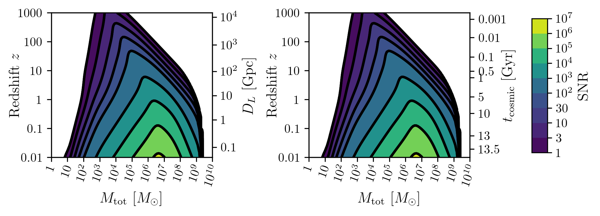
Another included feature is the ability to add luminosity distance or lookback times onto the right hand axes of the redshift vs. total mass plots.
figsize = get_fig_size()
fig, axes = plt.subplots(1,2,figsize=figsize)
wspace = 0.6
Plot_SNR('M',sample_x_array[-1],'z',sample_y_array[-1],SNR_array[-1],fig=fig,ax=axes[0],
         display=False,display_cbar=False,dl_axis=True,smooth_contours=False,
         xticklabels_kwargs={'rotation':70,'y':0.02},
         ylabels_kwargs={'labelpad':-3})
Plot_SNR('M',sample_x_array[-1],'z',sample_y_array[-1],SNR_array[-1],fig=fig,ax=axes[1],
         lb_axis=True,wspace=wspace,smooth_contours=False,
         xticklabels_kwargs={'rotation':70,'y':0.02},
         ylabels_kwargs={'labelpad':-3})
Changing Waveform Models
Thanks to swig wrapping, we can access the frequency domain waveforms
within lalsuite (specifically any found
here).
User beware though, this is mostly untested. Depending on the waveform
model, the SNR calculation could take much longer. To select between
waveforms, simply change the approximant either in the source
initialization, or inside the dictionary of extra parameters passed to
lalsuite.
#Number of SNRMatrix rows
sampleRate_y = 50
#Number of SNRMatrix columns
sampleRate_x = 50
#Variable on y-axis
var_y = 'z'
#Variable on x-axis
var_x = 'M'
lalsuite_kwargs = {"S1x": 0.5, "S1y": 0, "S1z": 0.2,
"S2x": -0.2, "S2y": 0.5, "S2z": 0.1,
"inclination":np.pi/2}
instrument = Initialize_LISA()
source = Initialize_Source(instrument,approximant='IMRPhenomPv3',lalsuite_kwargs=lalsuite_kwargs)
start = time.time()
[sample_x,sample_y,SNRMatrix] = snr.Get_SNR_Matrix(source,instrument,
var_x,sampleRate_x,
var_y,sampleRate_y)
end = time.time()
print('Model: ',instrument.name + '_' + var_x + '_vs_' + var_y,',',' done. t = : ',end-start)
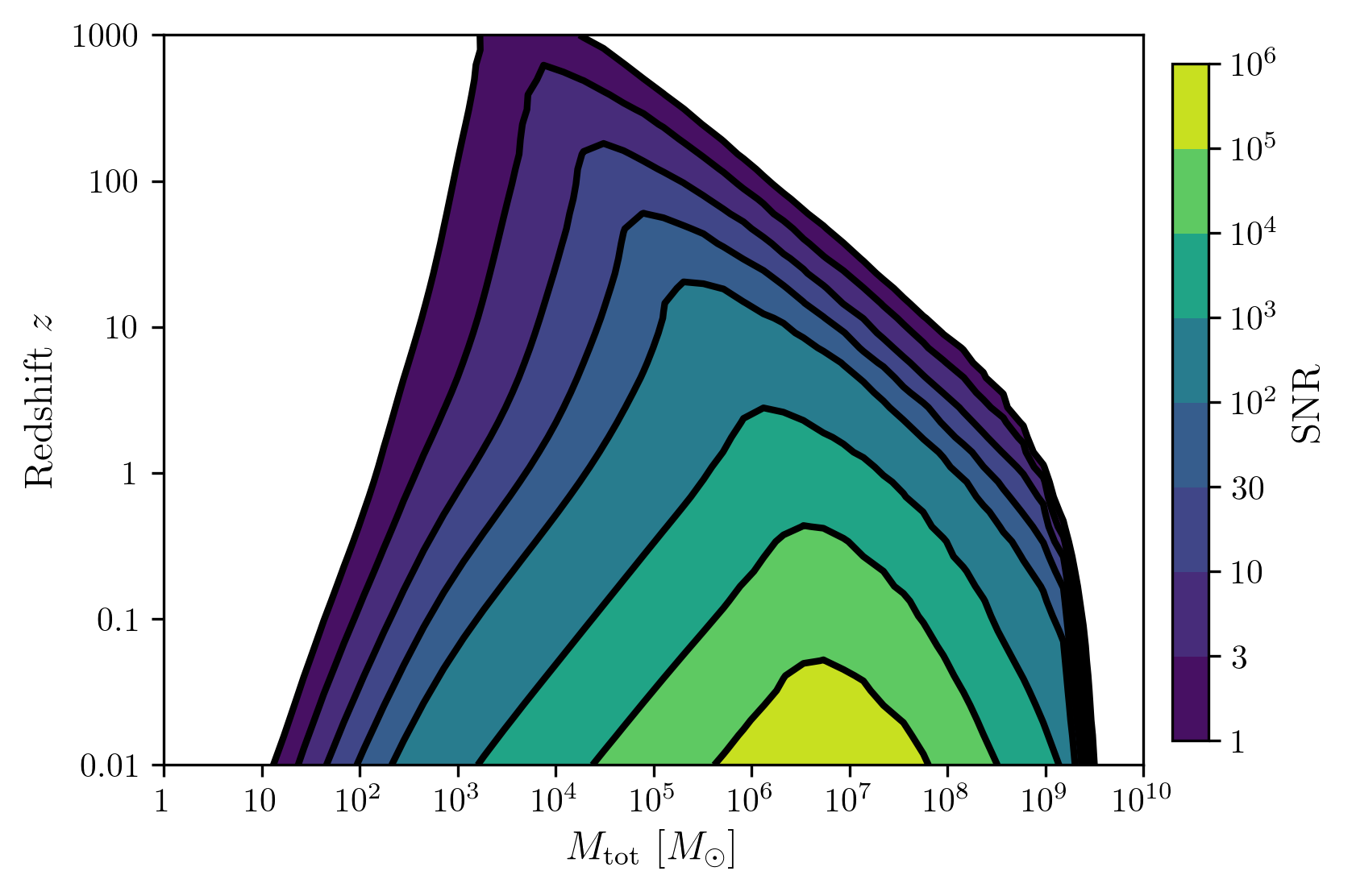
Plot_SNR(var_x,sample_x,var_y,sample_y,SNRMatrix,smooth_contours=False)
Model: LISA_prop1_M_vs_z , done. t = : 431.48117208480835
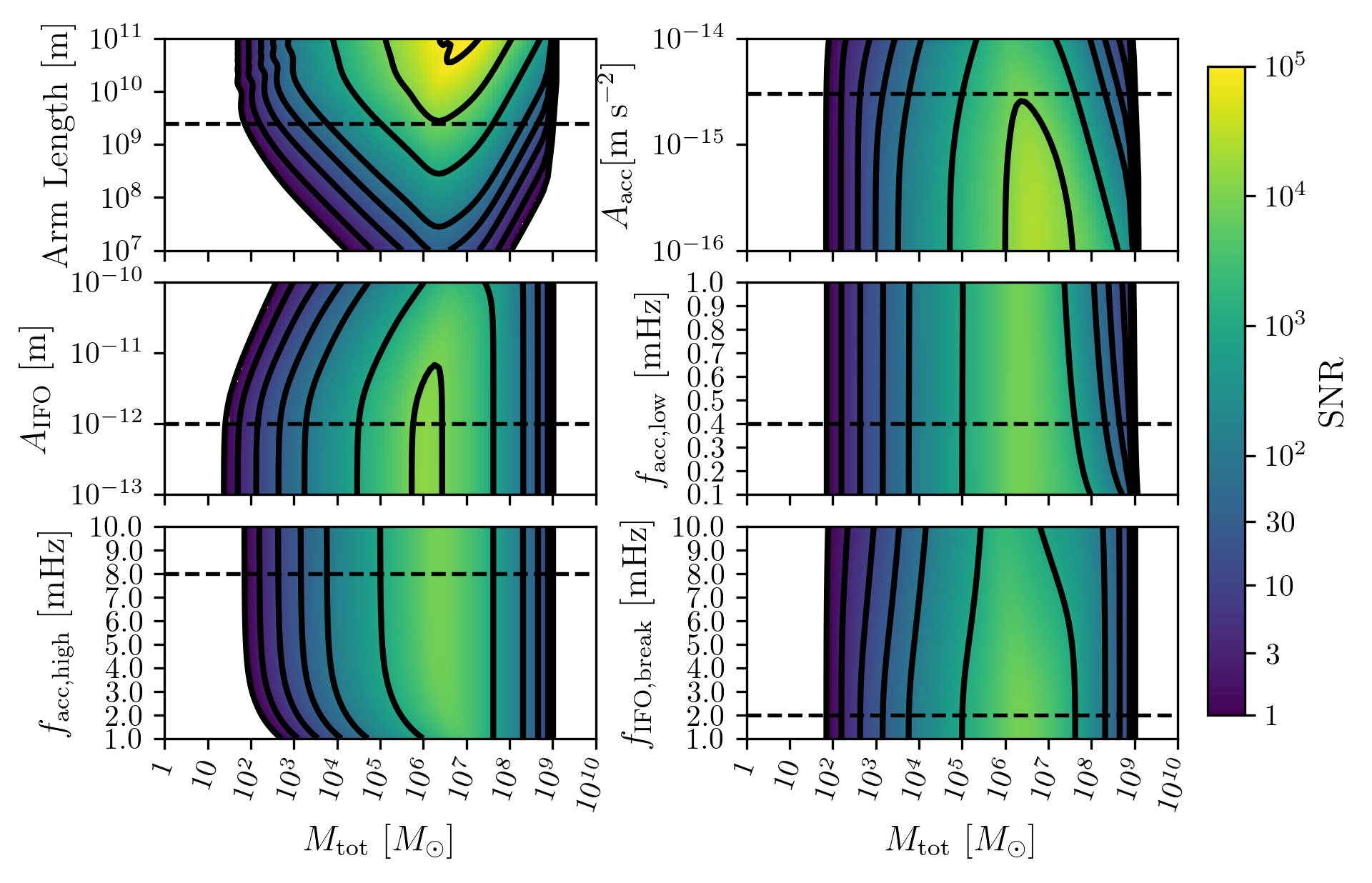
sampleRate_y = 100
sampleRate_x = 100
#Variable on y-axis
var_ys = ['L','A_acc','A_IFO','f_acc_break_low','f_acc_break_high','f_IFO_break']
#Variable on x-axis
var_x = 'M'
sample_x_array = []
sample_y_array = []
SNR_array = []
for var_y in var_ys:
    instrument = Initialize_LISA()
    source = Initialize_Source(instrument)
    start = time.time()
    [sample_x,sample_y,SNRMatrix] = snr.Get_SNR_Matrix(source,instrument,
                                                       var_x,sampleRate_x,
                                                       var_y,sampleRate_y)
    end = time.time()
    sample_x_array.append(sample_x)
    sample_y_array.append(sample_y)
    SNR_array.append(SNRMatrix)

    print('Model: ',instrument.name + '_' + var_x + '_vs_' + var_y,',',' done. t = : ',end-start)
Model:  LISA_prop1_M_vs_L ,  done. t = :  32.94680953025818
Model:  LISA_prop1_M_vs_A_acc ,  done. t = :  33.771636962890625
Model:  LISA_prop1_M_vs_A_IFO ,  done. t = :  33.917126417160034
Model:  LISA_prop1_M_vs_f_acc_break_low ,  done. t = :  34.29063296318054
Model:  LISA_prop1_M_vs_f_acc_break_high ,  done. t = :  34.608739614486694
Model:  LISA_prop1_M_vs_f_IFO_break ,  done. t = :  34.29920196533203
figsize = get_fig_size(scale=1.0)
fig, axes = plt.subplots(3,2,figsize=figsize)

#Can add lines on plot
fiducial_lines = [2.5e9,3e-15,1e-12,0.4*u.mHz.to('Hz'),8*u.mHz.to('Hz'),2*u.mHz.to('Hz')]
loglevelMax=5.0
hspace = .15
wspace = .35

ii = 0
for i in range(np.shape(axes)[0]):
    for j in range(np.shape(axes)[1]):
        if ii == (np.shape(axes)[0]*np.shape(axes)[1])-1:
            Plot_SNR('M',sample_x_array[ii],var_ys[ii],
                     sample_y_array[ii],SNR_array[ii],
                     fig=fig,ax=axes[i,j],display=True,display_cbar=True,
                     logLevels_max=loglevelMax,y_axis_line=fiducial_lines[ii],
                     hspace=hspace,wspace=wspace,
                     xticklabels_kwargs={'rotation':70,'y':0.02},
                     ylabels_kwargs={'labelpad':5})
        elif ii == (np.shape(axes)[0]*np.shape(axes)[1])-2:
            Plot_SNR('M',sample_x_array[ii],var_ys[ii],
                     sample_y_array[ii],SNR_array[ii],
                     fig=fig,ax=axes[i,j],display=False,display_cbar=False,
                     logLevels_max=loglevelMax,y_axis_line=fiducial_lines[ii],
                     hspace=hspace,wspace=wspace,
                     xticklabels_kwargs={'rotation':70,'y':0.02},
                     ylabels_kwargs={'labelpad':5})
        else:
            Plot_SNR('M',sample_x_array[ii],var_ys[ii],
                     sample_y_array[ii],SNR_array[ii],
                     fig=fig,ax=axes[i,j],display=False,display_cbar=False,
                     logLevels_max=loglevelMax,y_axis_line=fiducial_lines[ii],
                     x_axis_label = False,
                     hspace=hspace,wspace=wspace,
                     xticklabels_kwargs={'rotation':70,'y':0.02},
                     ylabels_kwargs={'labelpad':5})
        ii += 1
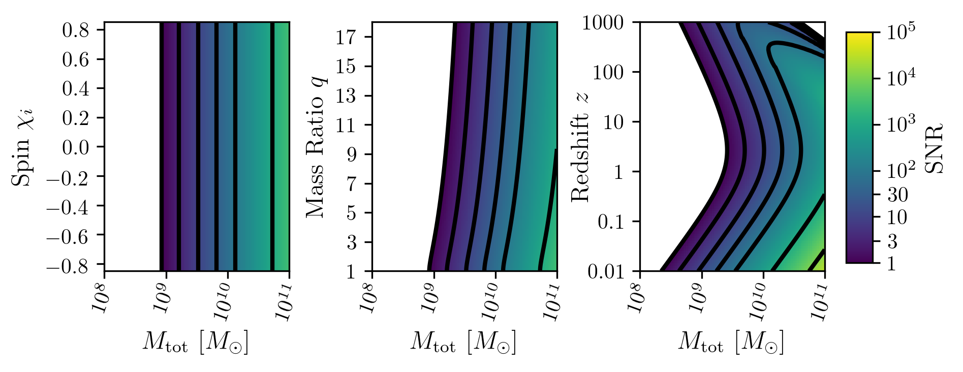
PTA SNRs
Same as the rest, just for example purposes!
#Variable on y-axis
var_ys = ['chi1','q','z']
#Variable on x-axis
var_x = 'M'
instrument = Initialize_NANOGrav()
sample_x_array = []
sample_y_array = []
SNR_array = []
for var_y in var_ys:
    source = Initialize_Source(instrument)
    start = time.time()
    [sample_x,sample_y,SNRMatrix] = snr.Get_SNR_Matrix(source,instrument,
                                                       var_x,sampleRate_x,
                                                       var_y,sampleRate_y)
    end = time.time()
    sample_x_array.append(sample_x)
    sample_y_array.append(sample_y)
    SNR_array.append(SNRMatrix)

    print('Model: ',instrument.name + '_' + var_x + '_vs_' + var_y,',',' done. t = : ',end-start)
Model:  NANOGrav_WN_M_vs_chi1 ,  done. t = :  24.73322606086731
Model:  NANOGrav_WN_M_vs_q ,  done. t = :  21.385414361953735
Model:  NANOGrav_WN_M_vs_z ,  done. t = :  22.074593544006348
figsize = get_fig_size()
fig, axes = plt.subplots(1,3,figsize=figsize)
loglevelMax=5.0
hspace = .1
wspace = .45

for i,ax in enumerate(axes):
    if i == (len(axes))-1:
        Plot_SNR('M',sample_x_array[i],var_ys[i],
                 sample_y_array[i],SNR_array[i],
                 fig=fig,ax=ax,display=True,display_cbar=True,
                 logLevels_max=loglevelMax,
                 hspace=hspace,wspace=wspace,
                 xticklabels_kwargs={'rotation':70,'y':0.02},
                 ylabels_kwargs={'labelpad':-5})
    else:
        Plot_SNR('M',sample_x_array[i],var_ys[i],
                 sample_y_array[i],SNR_array[i],
                 fig=fig,ax=ax,display=False,display_cbar=False,
                 logLevels_max=loglevelMax,
                 hspace=hspace,wspace=wspace,xticklabels_kwargs={'rotation':70,'y':0.02})
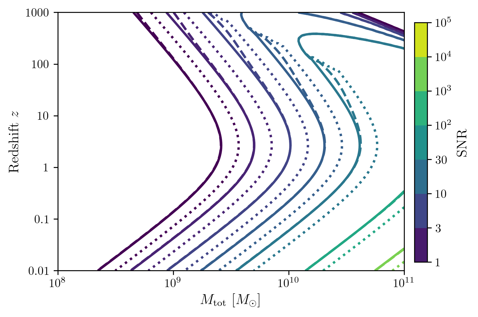
There is also functionality to plot two different plots together for eazy comparison. Here we compare the methods in the previous calculation to a source with an inclination of \(\pi/2\) and one using the alternate method of calculating the monochromatic strain with the phenomenological waveform amplitude.
instrument = Initialize_NANOGrav()
inc = np.pi/2
source = Initialize_Source(instrument)
[sample_x_inclined,sample_y_inclined,SNRMatrix_inclined] = snr.Get_SNR_Matrix(source,instrument,
                                                                              'M',sampleRate_x,
                                                                              'z',sampleRate_y,
                                                                              inc=inc)
[sample_x_PN_method,sample_y_PN_method,SNRMatrix_PN_method] = snr.Get_SNR_Matrix(source,instrument,
                                                                                 'M',sampleRate_x,
                                                                                 'z',sampleRate_y,method='PN')
fig,ax = plt.subplots()
Plot_SNR('M',sample_x_array[-1],'z',sample_y_array[-1],SNR_array[-1],
         display=False,display_cbar=False,fig=fig,ax=ax,
         contour_kwargs={'cmap':'viridis'},cfill=False)
Plot_SNR('M',sample_x_inclined,'z',sample_y_inclined,SNRMatrix_inclined,
         display=False,display_cbar=False,fig=fig,ax=ax,
         contour_kwargs={'cmap':'viridis','linestyles':':'},cfill=False)
Plot_SNR('M',sample_x_PN_method,'z',sample_y_PN_method,SNRMatrix_PN_method,fig=fig,ax=ax,
         contour_kwargs={'cmap':'viridis','linestyles':'--'},cfill=False)
These can take a long time if you vary the instrument parameters. Be careful with your sample rates!
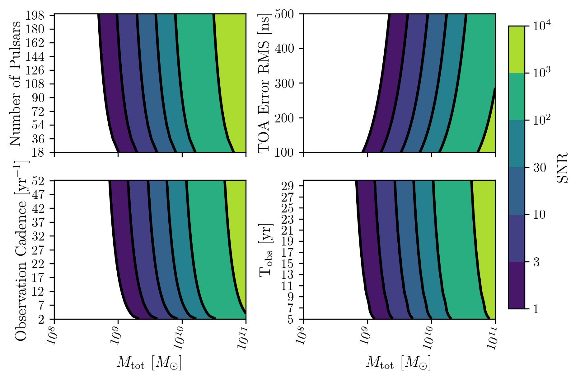
sampleRate_x = 50
sampleRate_y = 50
#Variable on y-axis
var_ys = ['n_p','sigma','cadence','T_obs']
#Variable on x-axis
var_x = 'M'
sample_x_array = []
sample_y_array = []
SNR_array = []
for var_y in var_ys:
    instrument = Initialize_NANOGrav()
    source = Initialize_Source(instrument)
    start = time.time()
    [sample_x,sample_y,SNRMatrix] = snr.Get_SNR_Matrix(source,instrument,
                                                       var_x,sampleRate_x,
                                                       var_y,sampleRate_y)
    end = time.time()
    sample_x_array.append(sample_x)
    sample_y_array.append(sample_y)
    SNR_array.append(SNRMatrix)

    print('Model: ',instrument.name + '_' + var_x + '_vs_' + var_y,',',' done. t = : ',end-start)
Model:  NANOGrav_WN_M_vs_n_p ,  done. t = :  134.68967270851135
Model:  NANOGrav_WN_M_vs_sigma ,  done. t = :  171.6554970741272
Model:  NANOGrav_WN_M_vs_cadence ,  done. t = :  172.50515484809875
Model:  NANOGrav_WN_M_vs_T_obs ,  done. t = :  261.6520907878876
figsize = get_fig_size(scale=1.0)
fig, axes = plt.subplots(2,2,figsize=figsize)

loglevelMax=4.0
hspace = .2
wspace = .3
smooth = False

ii = 0
for i in range(np.shape(axes)[0]):
    for j in range(np.shape(axes)[1]):
        if ii == (np.shape(axes)[0]*np.shape(axes)[1])-1:
            Plot_SNR('M',sample_x_array[ii],var_ys[ii],
                     sample_y_array[ii],SNR_array[ii],
                     fig=fig,ax=axes[i,j],
                     logLevels_max=loglevelMax,
                     hspace=hspace,wspace=wspace,
                     smooth_contours=smooth,
                     xticklabels_kwargs={'rotation':70,'y':0.02},
                     ylabels_kwargs={'labelpad':5})
        elif ii == (np.shape(axes)[0]*np.shape(axes)[1])-2:
            Plot_SNR('M',sample_x_array[ii],var_ys[ii],
                     sample_y_array[ii],SNR_array[ii],
                     fig=fig,ax=axes[i,j],display=False,display_cbar=False,
                     logLevels_max=loglevelMax,
                     hspace=hspace,wspace=wspace,
                     smooth_contours=smooth,
                     xticklabels_kwargs={'rotation':70,'y':0.02},
                     ylabels_kwargs={'labelpad':2})
        else:
            Plot_SNR('M',sample_x_array[ii],var_ys[ii],
                     sample_y_array[ii],SNR_array[ii],
                     fig=fig,ax=axes[i,j],display=False,display_cbar=False,x_axis_label=False,
                     logLevels_max=loglevelMax,
                     hspace=hspace,wspace=wspace,
                     smooth_contours=smooth,
                     xticklabels_kwargs={'rotation':70,'y':0.02},
                     ylabels_kwargs={'labelpad':2})
        ii += 1